
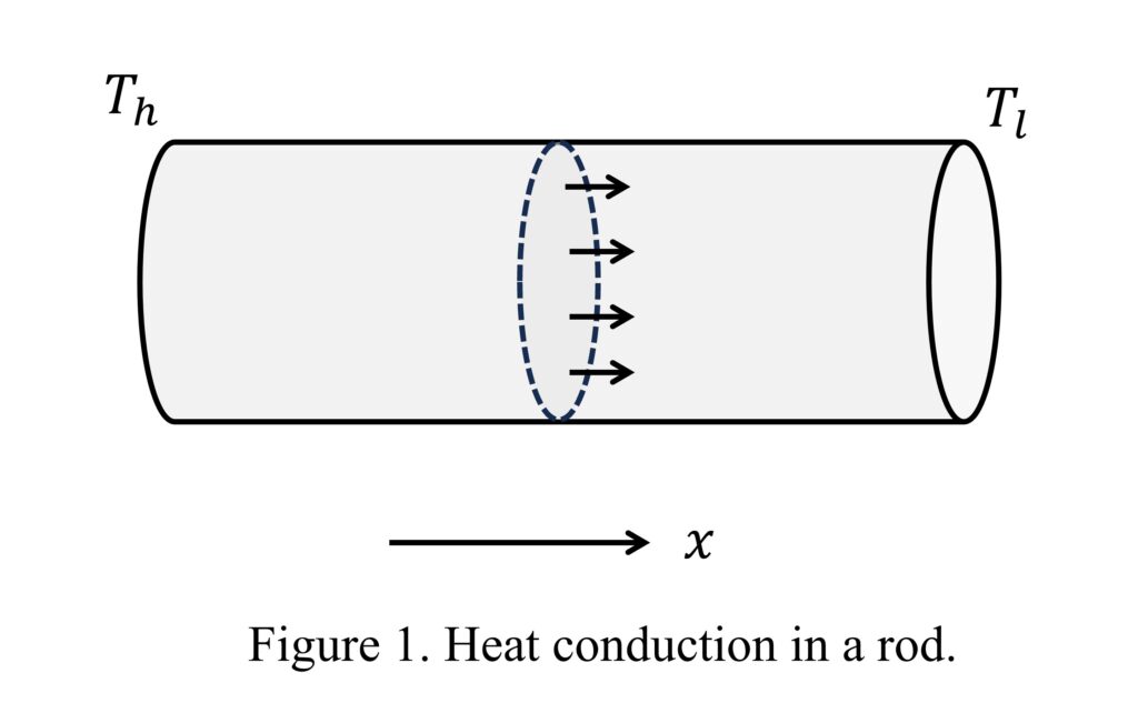
In science and engineering, we often need to study the transport of some physical quantities. One of the most straightforward examples is the transport of heat, as we all have experience with heat transfer. Imagine conducting an experiment where one end of a metal rod is held while the other end is heated. From experience, we know that heat will travel from the high-temperature end to the low-temperature end. Figure 1 illustrates this, with the high temperature denoted by \( T_h \) and the low temperature by \( T_l \).
By varying the conditions of the experiment, we can make the following observations:
- Observation 1: Increasing \( T_h \) results in faster heat transfer from the high-temperature end. Thus, the speed of heat transfer is proportional to the temperature difference.
- Observation 2: Increasing the length of the rod while maintaining the temperatures at both ends results in slower heat transfer. Therefore, the speed of heat transfer is inversely proportional to the length of the rod.
- Observation 3: The speed of heat transfer depends on the material of the rod. For instance, replacing the metal rod with a rubber one results in slower heating of the low-temperature end.
- Observation 4: The amount of heat transferred depends on time. Given sufficient time, even a rubber rod will eventually heat up at the low-temperature end.
- Observation 5: Heat always flows from high temperature to low temperature, but not the other way around.
Additionally, we can make the following claims, even though they are not directly observable:
- Claim 1: Consider a cross-sectional area as shown in Figure 1. If we break it into smaller pieces, the total heat passing through the entire area equals the sum of heat passing through each smaller piece.
- Claim 2: If we consider two different cross-sectional areas at different locations along the rod, we expect that the heat flowing through them will be, generally speaking, different. In other words, the amount of heat flowing through a cross-sectional area depends on the temperature difference at its location.
Since the amount of heat transferred depends on the area (Claim 1), it makes sense to focus on the heat transferred per unit area (thus we are essentially working with intensive quantities. See discussions in Topic 1 of the book). Additionally, since the amount of heat transferred depends on time (Observation 4), we should focus on a unit time interval. Indeed, the heat transferred per unit time conveys the speed of heat transfer necessary to describe Observations 1, 2, and 3. Given these considerations, we define heat flux, denoted by \( q \), as the amount of heat transferred across a surface per unit area per unit time.
Combining Observations 1 and 2, the speed of heat transfer, characterized by the heat flux, is proportional to \( \frac{\Delta T}{\Delta x} \). Claim 2 further clarifies that the temperature difference is actually the local temperature difference. This local temperature difference is equivalent to \( \frac{\Delta T} {\Delta x} \) as \( \Delta x \) approaches zero, or:
\[ q \propto \lim_{\Delta x \to 0} \frac{\Delta T}{\Delta x} = \frac{dT}{dx} \]
Based on Observation 3, we define a material constant, \( \kappa \), that characterizes the ability of a material to conduct heat. Denoting this constant as \( \kappa \), we have:
\[ q \propto \kappa \frac{dT}{dx} \]
Observation 5 suggests that heat flux is directional. To better describe the direction of heat flow, we define the positive \( x \) direction as from high temperature to low temperature (Figure 1). Since heat flows from high temperature to low temperature, \( q \) must be positive given our definition of positive direction. On the other hand, \( \frac{dT}{dx} \) is negative because \( T \) decreases as \( x \) increases. Thus,
\[ q \propto -\kappa \frac{dT}{dx} \]
Or:
\[ q = -c\kappa \frac{dT}{dx} \]
where \( c \) is a proportionality constant. Let \( c = 1 \), which is the most convenient. We can write:
\[ q = -\kappa \frac{dT}{dx} \]
This is known as Fourier’s law of heat conduction. We derived it based on our experimental observations and reasoning. The material constant, \( \kappa \), is known as the thermal conductivity.
So far, our discussion has been limited to one dimension. Heat can be transferred in different directions. In three-dimensional space, \( q \) becomes \( \vec{q} \), and \( \frac{dT}{dx} \) becomes the temperature gradient vector \( \nabla T \). Thus, the three-dimensional equation for heat conduction becomes:
\[ \vec{q} = -\kappa \nabla T \]
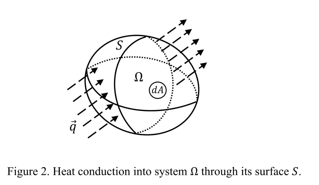
As defined, \( \vec{q} \) is the amount of heat conducted through a surface per unit area per unit time. To find the total amount of heat conducted per unit time into a system through its surface as shown in Figure 2, we need to integrate \( \vec{q} \) over surface \( S \). Depending on the direction of \( \vec{q} \), heat may flow into or out of the system \( \Omega \) (Figure 2). Following a similar process as described in Additional Exercise Problem 7, we have:
\[ Q = \iint_S -\vec{q} \cdot \vec{n} \, dA \]
where \( \vec{n} \) is the surface normal of \( dA \) and \( Q \) is the heat transfer rate (or the amount of heat transferred per unit time) into \( \Omega \).
As a quick exercise, consider the following questions:
- What is the dimension of \( \vec{q} \)? What about \( Q \)?
- What is the dimension of \( \kappa \)? What are typical values for metals? Plastics?
- Is \( Q \) a vector?
- Consider the cross-sectional area in Figure 1. What is the relation between \( q \) and \( Q \)?
Leave a Reply