
Suppose you deposit $100 in your bank account and then withdraw $10. At the same time, your account generates $1 in interest. The remaining balance is then $100 – $10 + $1 = $91$. This equation suggests that the balance in your account is equal to the amount you deposit, plus whatever interest is generated, and minus the amount you withdraw. This simple relation can be summarized as follows:
Money accumulation (account balance) = Money input (deposit) – Money output (withdraw) + Money generation (interest) (1)
We replaced the terms account balance, deposit, withdraw, and interest with money accumulation, money input, money output, and money generation, respectively. Of course, the idea remains the same. For example, depositing $100 into your bank account can also be viewed as $100 coming into your account. Your bank pays you $1 in interest, which is equivalent to $1 being generated in your account.
Now suppose you deposit $100 in your bank account every month and withdraw $10 every month. $1 is generated every month as interest. Then, you will accumulate $91 every month. In other words, the rate of balance accumulation is equal to the rate of deposit, plus the rate of interest generation, and minus the rate of withdrawal. Or:
Rate of money accumulation = Rate of money input – Rate of money output + Rate of money generation (2)
Indeed, the same idea can be applied to a broad range of physical quantities in science and engineering (this is why we changed our terminology from deposit to input, withdraw to output, and interest to generation). Suppose we are interested in a physical quantity for a system, and we can argue that the amount of that physical quantity in the system, or accumulation, is given by:
Accumulation = Input – Output + Generation (3)
Or, if we focus on the speed at which the amount of the physical quantity changes, we have:
Rate of accumulation = Rate of input – Rate of output + Rate of generation (4)
Equations (3) and (4) are known as the balance principle. Applied to money in your bank account, they become equations (1) and (2), respectively. Now, let’s apply the balance principle to the total mass of a system. In most cases, we are interested in the rate of mass change, and equation (4) becomes:
Rate of mass accumulation = rate of mass input – rate of mass output + rate of mass generation (5)
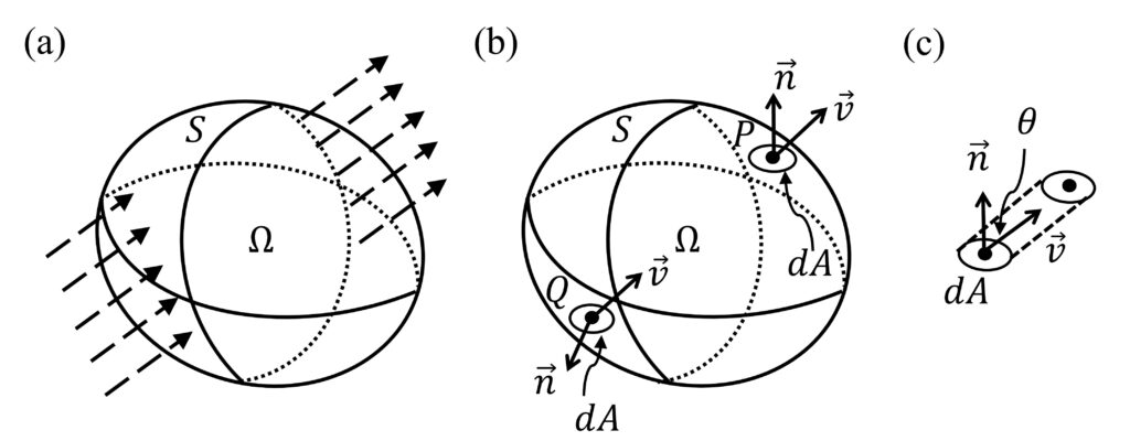
Figure 1. (a) An arbitrary volume ![]() , which is bounded by surface
, which is bounded by surface ![]() , within a flowing fluid. The flow velocity is indicated by the arrow. (b) An infinitesimal surface element
, within a flowing fluid. The flow velocity is indicated by the arrow. (b) An infinitesimal surface element ![]() at point
at point ![]() . The surface normal is given by
. The surface normal is given by ![]() and the flow velocity is given by
and the flow velocity is given by ![]() . The surface normal and flow velocity at a different point,
. The surface normal and flow velocity at a different point, ![]() , is also shown. (c) During an infinitesimal time
, is also shown. (c) During an infinitesimal time ![]() , the volume of the fluid flowing pass through
, the volume of the fluid flowing pass through ![]() is given by the volume of the slanted cylinder.
is given by the volume of the slanted cylinder.
Consider the total mass confined in volume \(\Omega\) whose surface is \(S\), as shown in Figure 1 above. If the density within \(\Omega\) is known, the total mass is given by:
\( M = \iiint_{\Omega} \rho \, d\Omega\) (6)
The derivative of Eq. (6) with respect to time is then the mass accumulation rate. In Additional Exercise Problem 7, we found an expression for the net mass inflow rate, which is the mass input rate minus the mass output rate. Additionally, we note that the rate of mass generation must be zero because mass cannot be generated. Thus, we have:
\( \frac{\partial}{\partial t} \iiint_{\Omega} \rho \, d\Omega = \iint_{S} -\rho \mathbf{v} \cdot \mathbf{n} \, dA \) (7)
Equation (7) is known as the integral mass balance equation. Applying Gauss’s divergence theorem (Topic 7 in the book), the right-hand side of Eq. (7) can be written as:
\(\iint_{S} -\rho \mathbf{v} \cdot \mathbf{n} \, dA = -\iiint_{\Omega} \nabla \cdot (\rho \mathbf{v}) \, d\Omega\) (8)
Thus, Eq. (7) becomes:
\(\iiint_{\Omega} \left( \frac{\partial \rho}{\partial t} + \nabla \cdot (\rho \mathbf{v}) \right) \, d\Omega = 0\) (9)
Because volume \(\Omega\) was arbitrarily chosen, the above integral is zero only if:
\(\frac{\partial \rho}{\partial t} + \nabla \cdot (\rho \mathbf{v}) = 0\) (10)
This is the well-known equation of continuity (or the differential mass balance equation), which has been derived using the balance principle. Continuity equations of other physical quantities can be similarly derived, and \(\rho\) is the density of the corresponding physical quantity, for example, charge density, probability density, etc.
Not all physical quantities are conserved. In such cases, a generation term must be added to Eq. (10). Let \(r\) be the rate of generation per unit volume, then we have:
\(\frac{\partial \rho}{\partial t} + \nabla \cdot (\rho \mathbf{v}) = r\) (11)
Equation (11) is equivalent to the convection-diffusion equation, Eq. (7.53), discussed in the book. Note that Eq. (7.53) in the book takes a slightly different form, where the net input rate includes contributions from both the velocity field and a gradient field.
Leave a Reply